Load the packages
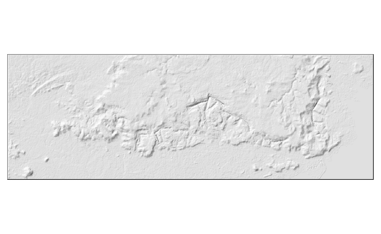
Prepare a base hillshade
Show code
bb <- c(82.48, 24.1, 82.8, 24.2) # extent for target site as left, bottom, right, upper

#dem <- getData(name = "SRTM", lon = 84, lat = 24, path = "./dem/") # download data from SRTM

#dem_crop <- dem %>% crop(extent(82.48, 82.8, 24.1, 24.2)) # cropped to target site
#rm(dem) # remove dem from environment

#slope <- terrain(dem_crop, opt= "slope") # extract slope from dem_crop
#aspect <- terrain(dem_crop, opt= "aspect") # extract aspect from dem_crop
#dem_hs <- hillShade(slope = slope, aspect = aspect, angle = 45, direction = 315) # prepare hill shade
# 45 altitude angle and 315 azimuth angle

#writeRaster(x = dem_hs, filename = "./data/dem_hs.tif", overwrite = T) # write to local directory
#rm(slope, aspect) # removed slope and aspect files

hs <- raster("./data/dem_hs.tif") # read the hillshade file

tm_shape(hs) +
      tm_raster(palette = "-Greys", n = 100, style = "cont", alpha = 0.7,
                         legend.show = FALSE)
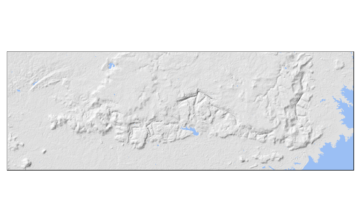
add water element
Show code
# https://storage.googleapis.com/earthenginepartners-hansen/GFC-2019-v1.7/Hansen_GFC-2019-v1.7_datamask_30N_080E.tif

#water <- raster("./data/Hansen_GFC2014_datamask_30N_080E.tif") %>%
      #crop(extent(82.48, 82.8, 24.1, 24.2)) %>%
      #calc(fun = function(x){x[x == 1] <- NA; return(x)})
#writeRaster(x = water, filename = "./data/singrauli-water.tif", overwrite = T) # write to local directory

water <- raster("./data/singrauli-water.tif") # read the hillshade file

# colors for water #4a80f5, #9bbff4, #a7cdf2, #AADAFF

tm_shape(hs) +
      tm_raster(palette = "-Greys", n = 100, style = "cont", alpha = 0.7,
                         legend.show = FALSE) + # hillshade
      tm_shape(water) +
      tm_raster(palette = c("#9bbff4"), style = "cat", legend.show = FALSE)  # water
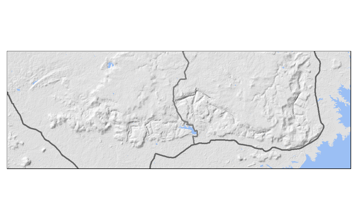
add major roads
Show code
#s_roads <- opq(bbox = bb) %>% # xmin, ymin, xmax, ymax
      #add_osm_feature(key = "highway", value = c("trunk")) %>%
      #osmdata_sf()
#s_roads <- s_roads$osm_lines
#st_write(s_roads, "./data/singrauli-road/singrauli-road.shp")

s_roads <- st_read("./data/singrauli-road/singrauli-road.shp")
Reading layer `singrauli-road' from data source
  `D:\R\abhikumar86.github.io\_posts\2021-07-21-singrauli-map\data\singrauli-road\singrauli-road.shp'
  using driver `ESRI Shapefile'
Simple feature collection with 30 features and 9 fields
Geometry type: LINESTRING
Dimension:     XY
Bounding box:  xmin: 82.4536 ymin: 24.08979 xmax: 82.77473 ymax: 24.20791
Geodetic CRS:  GCS_unknown
Show code
s_roads <- s_roads %>% st_set_crs(4326)

tm_shape(hs) + tm_raster(palette = "-Greys", n = 100, style = "cont", alpha = 0.7,
                         legend.show = FALSE) + # hillshade

      tm_shape(water) + tm_raster(palette = c("#9bbff4"), style = "cat",
                            legend.show = FALSE) + # water

      tm_shape(s_roads) + tm_lines(col = "ref", palette = c("grey50", "grey40"),
                                   lwd = 2.5, legend.col.show = FALSE) # roads
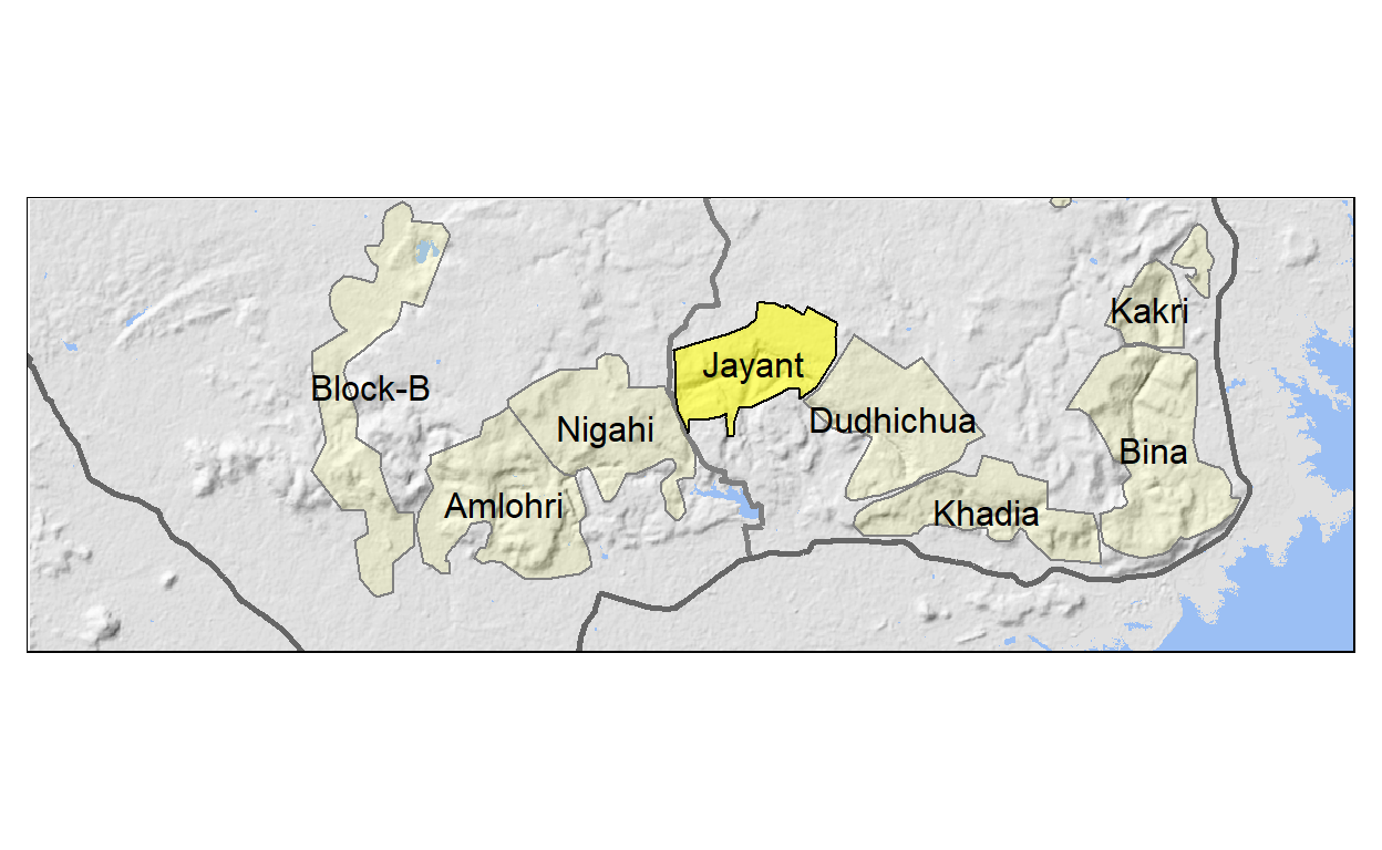
add coal mine boundaries
Show code
#s_mines <- opq(bbox = bb) %>% # xmin, ymin, xmax, ymax
       #add_osm_feature(key = "landuse", value = "quarry") %>%
       #osmdata_sf()
#s_mines <- s_mines$osm_polygons
#st_write(s_mines, "./data/singrauli-mines/singrauli-mines.shp")

# coal mines
cm <- st_read("./data/singrauli-mines/singrauli-mines.shp")
Reading layer `singrauli-mines' from data source
  `D:\R\abhikumar86.github.io\_posts\2021-07-21-singrauli-map\data\singrauli-mines\singrauli-mines.shp'
  using driver `ESRI Shapefile'
Simple feature collection with 10 features and 5 fields
Geometry type: POLYGON
Dimension:     XY
Bounding box:  xmin: 82.54869 ymin: 24.11217 xmax: 82.77247 ymax: 24.21588
Geodetic CRS:  GCS_unknown
Show code
cm$mine <- c("Khadia", "", "Bina", "Amlohri", "Dudhichua", "",
"Jhingurdah", "Kakri", "Nigahi", "Block-B")
# jayant mine
cmj <- cm %>% dplyr::filter(name == "Jayant Mine")
cmj$mine <- "Jayant"
tm_shape(hs) + tm_raster(palette = "-Greys", n = 100, style = "cont", alpha = 0.7,
legend.show = FALSE) + # hillshade
tm_shape(water) + tm_raster(palette = c("#9bbff4"), style = "cat",
legend.show = FALSE) + # water
tm_shape(s_roads) + tm_lines(col = "ref", palette = c("grey50", "grey40"),
lwd = 2.5, legend.col.show = FALSE) + # roads
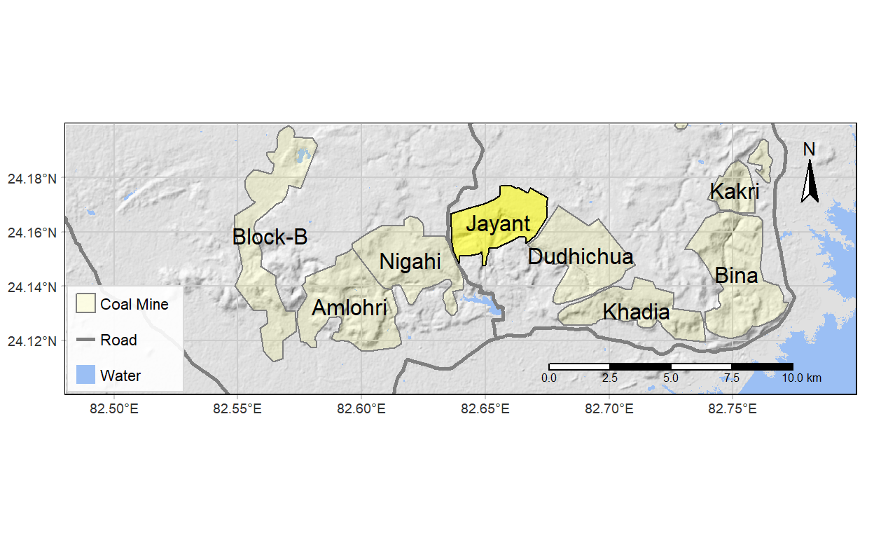
tm_shape(cm) +
tm_fill(col = "yellow", alpha = 0.1) +
tm_borders(col = "grey50") +
tm_text(text = "mine") + # coal mine shapes
tm_shape(cmj) + tm_fill(col = "yellow", alpha = 0.5) +
tm_text(text = "mine") +
tm_borders(col = "black") # Jayant Mine shape
prepare inset map
https://map.igismap.com/gis-data/india/administrative_state_boundary?utm_source=website&utm_medium=datadownload&utm_campaign=india
https://map.igismap.com/gis-data/india/administrative_assembly_constituencies_boundary?utm_source=website&utm_medium=datadownload&utm_campaign=india
Show code
# https://www.naturalearthdata.com/download/50m/cultural/ne_50m_admin_0_countries.zip
world_adm <- st_read("D:/spatial-data/admin/ne_world_adm/ne_50m_admin_0_countries.shp")
Reading layer `ne_50m_admin_0_countries' from data source
  `D:\spatial-data\admin\ne_world_adm\ne_50m_admin_0_countries.shp'
  using driver `ESRI Shapefile'
Simple feature collection with 241 features and 94 fields
Geometry type: MULTIPOLYGON
Dimension:     XY
Bounding box:  xmin: -180 ymin: -89.99893 xmax: 180 ymax: 83.59961
Geodetic CRS:  WGS 84
Show code
# Indian states
ind_adm <- st_read("D:/spatial-data/admin/ind_adm1/ind_adm1.shp")
Reading layer `ind_adm1' from data source
  `D:\spatial-data\admin\ind_adm1\ind_adm1.shp' using driver `ESRI Shapefile'
Simple feature collection with 37 features and 4 fields
Geometry type: MULTIPOLYGON
Dimension:     XY
Bounding box:  xmin: 68.09348 ymin: 6.754368 xmax: 97.4115 ymax: 37.07761
Geodetic CRS:  WGS 84
Show code
# https://map.igismap.com/gis-data/india/administrative_outline_boundary?utm_source=website&utm_medium=datadownload&utm_campaign=india

ind_adm0 <- st_read("D:/spatial-data/admin/ind_adm0/ind_adm0.shp")
Reading layer `ind_adm0' from data source
  `D:\spatial-data\admin\ind_adm0\ind_adm0.shp' using driver `ESRI Shapefile'
Simple feature collection with 1 feature and 4 fields
Geometry type: MULTIPOLYGON
Dimension:     XY
Bounding box:  xmin: 68.18625 ymin: 6.755953 xmax: 97.41529 ymax: 37.07827
Geodetic CRS:  WGS 84
Show code
#s_bb <- bb_poly(hs, projection = 4326) # bounding box

s_bb <- st_bbox(obj = c(xmin = 81.5, xmax = 83.5, ymin = 23.5, ymax = 24.5),
                    crs = st_crs(hs)) %>%
      st_as_sfc()

inset_map <- tm_shape(world_adm, bbox = st_bbox(ind_adm)) +
      tm_fill(col = "grey95") +

      tm_shape(ind_adm) + tm_fill(col = "grey90") + tm_borders(col = "grey70", lwd = 0.5) +

      tm_shape(ind_adm0) + tm_borders(lwd = 0.75) +

      tm_shape(s_bb) + tm_borders(col = "red", lwd = 0.75) +

      tm_layout(bg.color = "#9bbff4", frame = "grey85")

#rm(cm, cmj, hs, ind_adm, ind_adm0, s_bb, s_roads, water, world_adm) # remove undesired files
aspect ratios for main map and inset map
Show code
# aspect ratio for main map
xy <- st_bbox(hs)
asp <- (xy$ymax - xy$ymin)/(xy$xmax - xy$xmin)

# aspect ratio inset map
xy <- st_bbox(ind_adm)
asp2 <- (xy$ymax - xy$ymin)/(xy$xmax - xy$xmin)
final main map
Show code
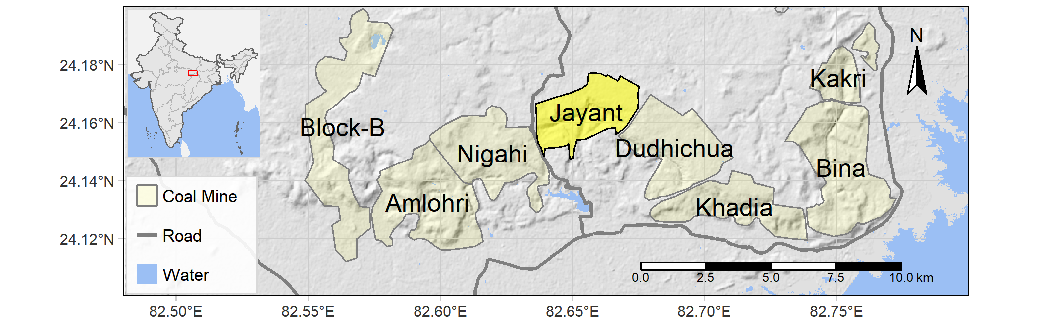
main_map <- tm_shape(hs) +
      tm_raster(palette = "-Greys", n = 100, style = "cont", alpha = 0.7,
                legend.show = FALSE) + # hillshade

      tm_graticules(col = "grey80") + # graticules

      tm_shape(water) +
      tm_raster(palette = c("#9bbff4"), style = "cat", legend.show = FALSE) + # water

      tm_shape(s_roads) +
      tm_lines(col = "grey50", lwd = 2.5) + # roads

      tm_shape(cm) +
      tm_fill(col = "yellow", alpha = 0.1) +
      tm_borders(col = "grey50") +
      tm_text(text = "mine") + # coal mine shapes

      tm_shape(cmj) + tm_fill(col = "yellow", alpha = 0.5) +
      tm_text(text = "mine") +
      tm_borders(col = "black") + # Jayant Mine shape

      tm_compass(position = c("right", "top")) + # North Arrow

      tm_scale_bar(position = c(0.6, 0.015), breaks = c(0, 2.5, 5, 7.5, 10)) + # scale

      tm_add_legend(type = "fill", labels = "Coal Mine", col = "yellow", alpha = 0.1,
                    border.col = "grey50") + # mine legend
      tm_add_legend(type = "line", labels = "Road", col = "grey50", lwd = 2.5) + # road legend
      tm_add_legend(type = "fill", labels = "Water", col = "#9bbff4", border.col = NA) + # water legend

      tm_layout(legend.position = c(0.0035, 0.01), legend.width = 0.6, legend.height = 0.6*asp2,
                legend.bg.color = "white", legend.bg.alpha = 0.9,
                legend.text.size = 0.75, legend.frame = "grey85")

main_map
arrange and save the final maps
# Create viewport
vp <- viewport(x = 0.115, y = 0.98, width = unit(1, "inches"),
               height = unit(1*asp2, "inches"), just = c("left", "top"))

# save the map
tmap_save(main_map, filename = "./data/singrauli-map.png", insets_tm = inset_map,
          insets_vp = vp, height = asp*7, width = 7, units = "in", dpi = 300)

# save map in pdf
tmap_save(main_map, filename = "./data/singrauli-map.pdf", insets_tm = inset_map,
          insets_vp = vp, height = asp*7, width = 7, units = "in", dpi = 300)
Show code
Corrections
If you see mistakes or want to suggest changes, please create an issue on the source repository.
Reuse
Text and figures are licensed under Creative Commons Attribution CC BY 4.0. Source code is available at https://github.com/abhikumar86/abhikumar86.github.io/, unless otherwise noted. The figures that have been reused from other sources don't fall under this license and can be recognized by a note in their caption: "Figure from ...".
Citation
For attribution, please cite this work as
Kumar (2021, July 21). Abhishek Kumar: Singrauli Map. Retrieved from https://abhikumar86.github.io/posts/2021-07-21-singrauli-map/
BibTeX citation
@misc{kumar2021singrauli,
  author = {Kumar, Abhishek},
  title = {Abhishek Kumar: Singrauli Map},
  url = {https://abhikumar86.github.io/posts/2021-07-21-singrauli-map/},
  year = {2021}
}